Ease in/out-linear interpolation implemented incorrectly

I’ve been trying to untangle the mathematics behind various interpolations and I’ve come across a rather serious issue. It seems that the linear interpolation is implemented incorrectly, at least with the ease in/out interpolation.

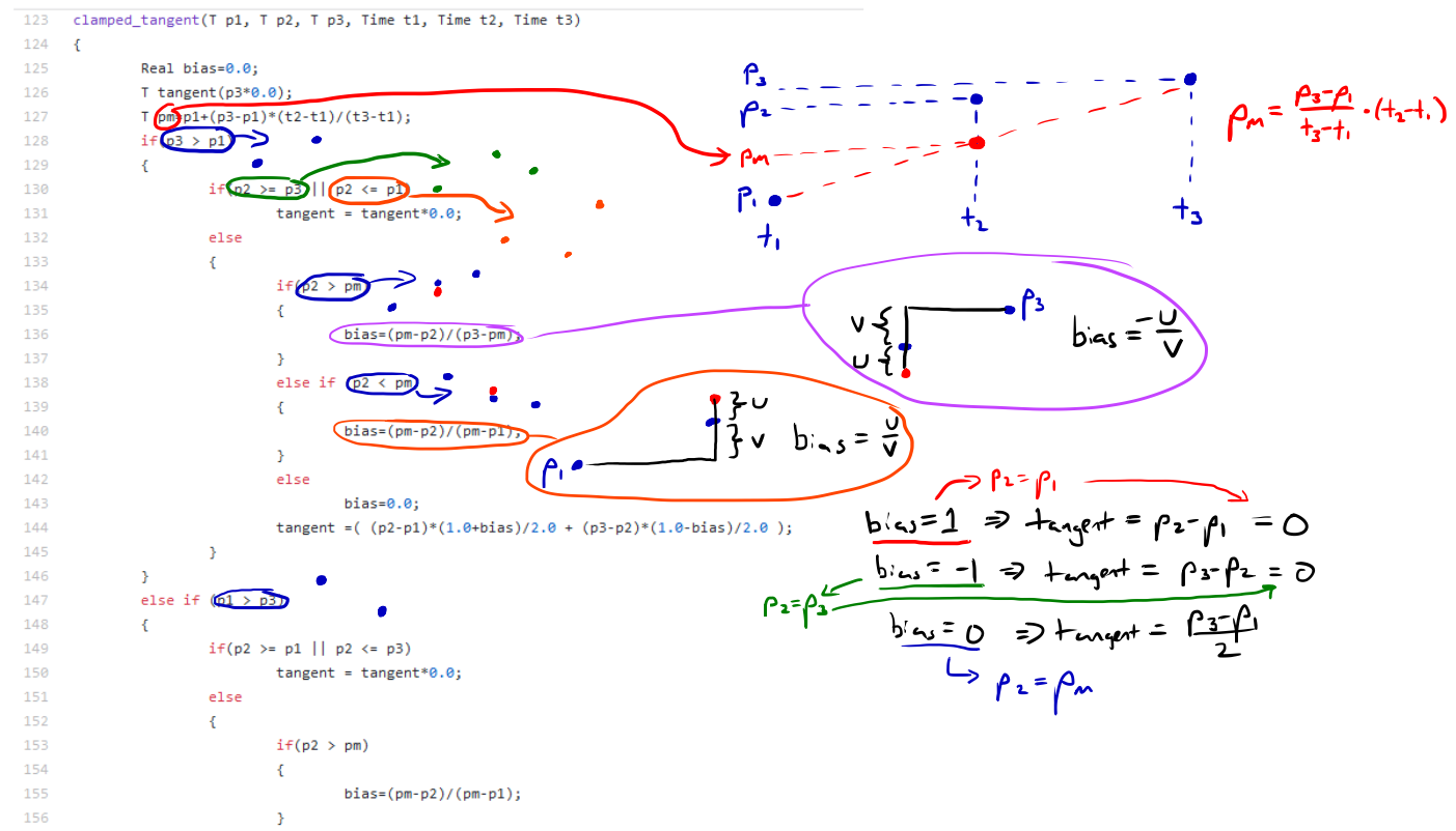
As far as I can tell, all interpolations except constant are given by a cubic spline, which is to say that they are governed by the differential equation y’’’’ = 0 (see the topic I linked to for a somewhat more detailed treatment of the subject). The only difference between the interpolations should be the boundary conditions. The linear interpolation has no cubed or squared terms, and so it appears to be implemented slightly differently effectively with the differential equation y’’ = 0 and boundary conditions something like y(0) = y_0, y’(t_f) = (y_f-y_0)/(t_f-t_0). (I’m not sure if this is actually what’s going on “under the hood”, but I’ll show in a moment that something is going wrong.)

We expect that when we use some waypoint at one end and a linear waypoint at the other end, the value should change in a, you know, linear fashion near its final time. How would we model this mathematically? We expect y’’(t_f) = 0.

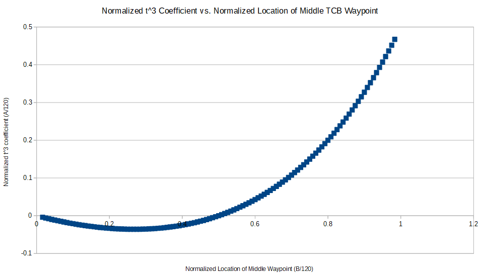
Is that what we see? In a word, no. I set an ease in/out waypoint at frame 0 with a value of 0 and a linear waypoint at frame 100 with a value of 1 and tabulated the values in Excel (actually LibreOffice Calc). Here’s the resulting graph:

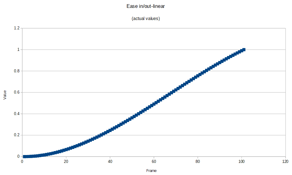
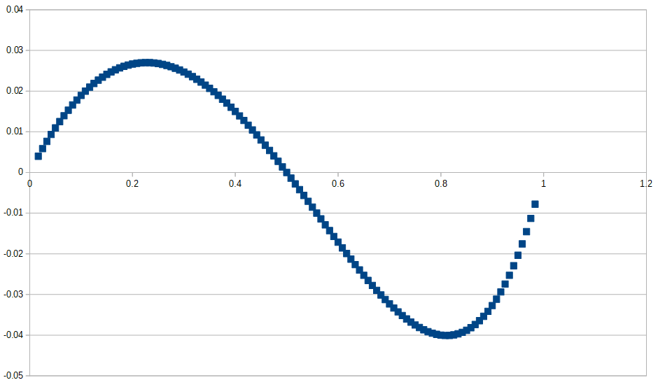
This may not look bad at first glance. The left end certainly reflects the ease in/out waypoint, but a close look at the right end only looks linear-ish. In fact, it looks like it’s tapering off slightly. I confirmed this by graphing the derivative:

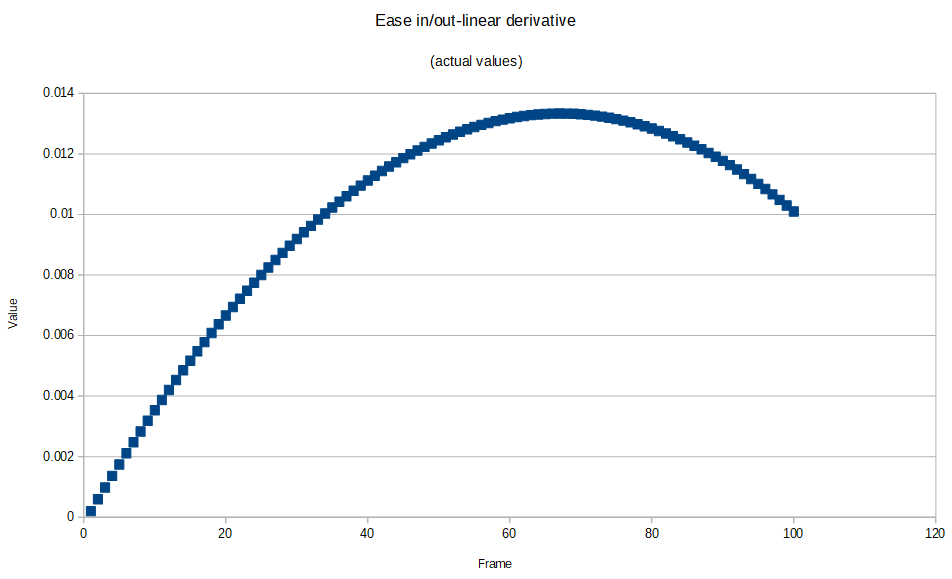
Blech. A linear interpolation should produce a constant derivative at its right end. That parabola being graphed should reach its maximum at frame 100.

Here’s what I propose the interpolation should actually look like:

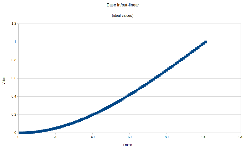
Much better! It’s easing in from the left end and it looks nice and linear at the right end. Let’s also graph the derivative to confirm that this is correct:

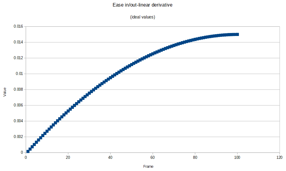
Note how the derivative is constant near frame 100, as we would hope.

This latter function was produced by changing the boundary conditions to:
y(0) = 0
y’(0) = 0
y(100) = 1
y’’(100) = 0

That last boundary condition is the only one that was changed. Note that it is now based on the second derivative.

How do we fix this? I’ll be honest: this is a real mess. If we were to suddenly change the linear interpolation, then every animation made before the change with a (something)-linear interpolation will be affected, possibly ruining those animations. I propose the new, correct interpolation be phased in slowly. First, we introduce “new linear” as an interpolation. Then, in a subsequent revision, we relable the current (broken) linear interpolation “legacy linear”. In the following revision, we relabel “new linear” to “linear” and make a warning box pop up warning users whenever they use it that the legacy linear interpolation is being deprecated soon. Finally, some years down the line, we scrap the legacy linear interpolation entirely and leave it to users to correct their animations as necessary.

I can’t seem to remember my credentials for the bug report site, so I kindly ask that someone submit this there. I hope I’ve made it clear that this is a rather serious issue and if you think it’s not a big deal, I’ll try to do a better job of explaining why this is oh-so-very-wrong.

I’m continuing my investigation into other interpolations.

2 Likes

Could you investigate the code I pointed to you?

I’m looking into it occasionally. I just deciphered the clamped_tangent function defined starting line 123. I see that p_m is interpolated at t_2 from (t_1, p_1) and (t_3, p_3), then a number of different cases are considered. If p_2 lies outside of p_1 and p_3, tangent is zero. If it’s exactly on p_2, tangent is (p3-p1)/2. If p_2 is less than pm (closer to p_1), bias is positive and if p_2 is greater than p_m (closer to p_3), bias is negative. I assume this is to produce a cubic spline that smoothly connects p_1, p_2, and p_3.

The only problem is I don’t know where in the code “tangent” is used. What does it mean? I also see lots of references to waypoint-waypoint connections, but I’m not yet ready to work on that. You linked to line 397 and I’ll get to it eventually.

I put together some figures to annotate the code. I think it would be nice to eventually produce an animation explaining the underpinnings of Synfig.

I might have the answer, although my programming skills aren’t the greatest and I haven’t double-checked the math.

[Edit: I screwed up. In a previous version of this post, I accidentally used BC p’‘(1)=1 instead of p’'(1)=0. I’ve corrected it and am now much more confident in my answer. At least I wrote the disclaimer above.]

Here’s the relevant code, starting at line 566:

  				    if(
  					next_get_before==INTERPOLATION_LINEAR || next_get_before==INTERPOLATION_HALT ||
  					(next_get_before==INTERPOLATION_TCB && after_next==animated.waypoint_list_.end()) ||
  					(next_get_before==INTERPOLATION_CLAMPED && after_next==animated.waypoint_list_.end())
  					)
  				{
  					/// t2 = p2 - p1
  					curve.second.t2()=subtract_func(curve.second.p2(),curve.second.p1());
  				}

The tangent is set to p2-p1, which gives rise to the funky behavior I indicated above. I propose the following modification, separating the ease-linear case from others:

  				    if(
  					iter_get_after==INTERPOLATION_EASE && next_get_before==INTERPOLATION_LINEAR
  					)
  				{
  					/// t2 = 3/2*(p2 - p1)
  					curve.second.t2()=3/2*subtract_func(curve.second.p2(),curve.second.p1());
  				}

The factor of three-halves seven-fourths is what I came up with in reverse engineering the cubic Hermite spline function.

Line 511 or thereabouts would need to be correspondingly changed to cover the linear-ease case. It probably should be t1 = 3/2*(p2-p1), but I could be wrong. I’ll need to check it.

It’s overwhelmingly likely that TCB-linear and clamped-linear would need to be changed as well for much the same reason-- we expect p’'(t) = 0 near a linear waypoint.

I’ve found another potential issue with the TCB-TCB spline when the spline segment is at either end. At the initial and final spline segments, all three TCB parameters are thrown out the window and the tangent is just p_1-p_0 or p_N-p_N-1, where p_0 and p_N are the first and last values. This gives us full control over the tangents in the interior waypoints but no control over the tangents at endpoints. Wouldn’t it be nice to have them still dependent on the parameters we set? In its current implementation, we could have a very large T, C, or B throughout the spline’s interior and then get behavior inconsistent with that at the endpoints.

This stackexchange post indicates that to handle endpoint cases, the second derivative is often set to 0 (natural BC), which is ironically the very same solution I suggest for the linear case. I’ll need to check that this is compatible with altering the the T, C, and B parameters, plus look into the mathematics of how this spline might be defined.

Sorry I keep bumping this thread, especially since I’m expanding its scope. I’ve found a new problem/mystery. So far, I’ve learned a lot about how the TCB waypoint works and shown that my own equations are consistent with what Synfig produces. I’ll write up my findings at a later date, when I have a more complete understanding.

I’m trying to figure out how the TCB waypoint works when it is collinear with surrounding TCB waypoints. I produced a very simple animation in which a parameter (opacity) takes the value 0 at frame 0, 120 at frame 120, and 80 at frame 80 (to be varied), each with an associated TCB waypoint. All three parameters were set to 0, so it’s “vanilla” TCB.

Graphically, here’s what comes out:

It doesn’t seem too weird, but if you look closely at that middle waypoint, it does not appear that the derivative is constant and instead the curve “drapes down” slightly between the pairs of waypoints. Eh? With continuity set to 0, shouldn’t the derivative be continuous?

You’ll notice I included values to the left, confirming this issue. In the image above, the middle TCB waypoint has value 80 at frame 80 and it currently displays frame 40. A linear function-- what seems sensible to me-- would produce an opacity value of 40 at frame 40, yet we’re a whole 1.25 short and it’s around 38.75 (I strongly suspect the last digit in the screenshot is a rounding error).

None of this is outright shocking to me because I accept that the TCB waypoint might run into issues over non-uniform time domains, but what I can’t wrap my head around is where the damn numbers come from. The problem disappears entirely when I put the middle waypoint at frame 60 (and value 60) and gets worse as you move it closer to the waypoints at either side. I did some curve fitting for the values and used that to deduce the incoming tangent (basically the derivative of this function just before the middle waypoint frame, except normalized to time interval [0,1]). I have a few other values that are non-integers that I’ll omit, but some values of interest include:
frame: 60 … tangent: 60
frame: 80 … tangent: 90
frame: 90 … tangent: 108
frame: 96 … tangent: 120

(For emphasis, we expect that with a linear function, those frames and tangents should be equal.)

That’s part of what makes this so frustrating: the fact that there are a handful of integer values suggests there is a nice, elementary math function to explain this but despite toying with the numbers for a few hours, I’m stumped.

I know user engagement in this thread hasn’t been very high, but does anyone have any idea what might be going on?

2 Likes

Although I’m not replying anything here for now, I’ve been reading your posts because it will help me to resume my work on letting user to set TCB “parameter” (actually the indirect tangents) as they were bézier, as proposed by Konstantin.

But right now my focus is fix some copy and paste errors (including skeleton) and a new color dialog to solve a minor but annoying issue. I hope in time to 1.4.1 release.

As this code is really tricky I can’t really properly analyze it now :frowning: Besides any change here would break every animation/synfig file that currently use this broken(?)/wrong(?)/unexpected(?) behavior.
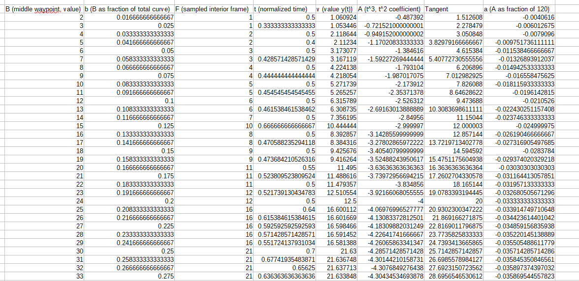
1 Like

Nice addition you’re working on! Personally, I’m not sure how the handles will jibe with the T, C, and B parameters. I would propose that we should introduce a new waypoint to avoid the TCB parameters entirely, but I actually like that Synfig doesn’t have too many waypoint styles; introducing another one might just be confusing.

Incidentally, I haven’t yet investigated the “temporal tension” parameter. I assume that with T, C, B, and TT, this gives us enough degrees of freedom to uniquely reverse-engineer any pair of tangents. (On further thought, at each TCB waypoint, only the tangents in and out need be specified, which should be two degrees of freedom and the system is perhaps overdetermined. This stuff is very confusing.) The only extent to which I’ve looked at temporal tension is on the wiki page where it’s apparent that when TT is set to 5, the curve is no longer cubic but at least 6th degree. That strikes me as so unusual that I question whether there’s some error here.

That actually relates to why I was investigating the TCB waypoint in the first place. I was hoping to determine how to simulate a “true linear” waypoint using TCB. I’m stuck because I don’t know why TCB acts this way when it’s not exactly halfway between two other waypoints, but for what it’s worth, when you have a TCB waypoint sandwiched exactly halfway between two ease in/out waypoints, you can use T=-0.5 and C=-1 to make the second derivative vanish in the proximity of the TCB waypoint. I didn’t include this in my previous post because I wanted to stick to the issue and not get bogged down in personal narrative.

Regarding your own issue, I’m not sure if this is where you’re running into trouble or whether the equations involving T, C, and B are invertible, but if they aren’t, I’d go with Newton’s method for inverting it. I can also think of some issues with treating these time curves like Bezier curves, most serious of which is that if we impose too many boundary conditions, I suspect the solutions might not be stable. Just throwing that out there.

Finally, I’ve given more thought as to how to introduce changes to waypoint definitions. I think the best thing to do would to have a separate tab under canvas properties that allows the user to select between new and legacy definitions, maybe with a short warning above stating that the default definitions will change to “new” with the next version of Synfig.

Thanks for brainstorming with me!

1 Like

Rodolfo, would you be able to help me briefly with line 550? I don’t know enough C++ to decipher it myself anytime soon. It just strikes me as inconsistent with the previous two lines. What I’m most confused by is why it says “get(T())” near the end of the line when I think it should say something like “get(p())”. I know the variable names may be inconsistent, but I would guess that T is in reference to the tangent while p should be the value. I have a poor understanding overall, though.

If the TCB function were working correctly as I understand it, the tangent would always be (p3-p1)/2 whenever T=C=B=0 (i.e., it should always be 60 for my previous example with a linear growth from 0 to 120 over 120 frames). That strikes me as unusual, since we want it to change as we move the middle waypoint. On the other hand, some behavior of the TCB waypoint is unusual but correct. I think much of this arises from the fact that it’s usually presented in the context of graphical splines while here we’re using it to define a one-dimensional function. For example, Wikipedia’s article includes a figure that indicates the spline reduces to straight line segments when T=1. When we use T=1 in Synfig, we instead see that the derivative of the function goes to zero and the waypoint acts identical to an ease in/out waypoint. Inspecting the math reveals that Synfig is correct (at least in this regard) and the confusion arises because our horizontal coordinates for our spline come directly from t(ime), not from a parameterized cubic spline dependent on the same values of T, C, and B.

The notation usually means:

Pc : Current Point
Pp: Previous Point
Pn: Next Point

Well, trying to being not too technical: no problem here.
In some details:
getValue() returns a ValueBase data type (it is a synfig variable type of a non-‘constrained’ type, ie. it can contains an integer, a real number, a string, etc - but one value at a time).
The .get() is how you get a typed-value (as C++/C/Java are typed languages). Instead of having getInteger(), getReal(), getString(), etc, there is one single method called get(), whose parameter is any variable to indicate what is the desired type. The parameter contents aren’t used neither set in the get() call.

But-- if I understand this correctly-- you can confirm that T is the appropriate value to be loaded and not, as I would guess, a tangent?

Edit: You can disregard most of the below. I found the rational function that gives rise to the tangents we see. Let L be the length of the total time interval and b be the fraction of the total interval where you place the middle TCB waypoint. For example, if the first and last TCB waypoints are placed at 0 and 120 and the middle waypoint is placed at 40, then L=120 and b=40/120=1/3=0.333333. The t^3 coefficient in the spline from the first waypoint to the middle is then A = -L*b*(2b-1)/(2b-4). For example, if L=120 and b=80, we find A=-1202/3(4/3-1)/(4/3-4)=-80*(1/3)/(-8/3)=80*1/8=10. The tangent is then T=B+A=90. Next, I need to find out why this is what the code outputs instead of 0, the sensible value.

I revisited the TCB funny business and am going to attempt a more detailed write-up as I’d like people to be able to follow along with my findings and reproduce them. I realized that the curve fitting I was doing when I last brought this up was overkill because there’s only one degree of freedom: the tangent. That means I can avoid the tedium of curve fitting and instead tabulate just one value at a time, allowing me to investigate this phenomenon over its full range.

  1. Open a new animation and create TCB waypoints for some (scalar, real) object at 0 and 120 frames. Set the corresponding values for these waypoints to 0 and 120, respectively. This produces a straight line between the two waypoints, giving values y(t) = t. (Linear waypoints also do the trick for this analysis.)

  2. Add a third TCB waypoint somewhere between the two. I’ll call its position B. Give it the corresponding value of B as well while leaving tension, continuity, and bias parameters at 0. Unless you happened to choose B=60, the plot is no longer linear. You can confirm this by selecting any frame other than your three waypoints, noting that the value is no longer equal to the frame. This is the issue I’m currently investigating.

  3. We wish to quantify this phenomenon. The cubic spline is given most generally by y(t) = at^3 + bt^2 + ct + d, where t is the normalized time (0<t<1). Our left endpoint is defined to be 0 by the first waypoint, so d is zero. The outgoing tangent from the first waypoint is also nicely defined as B because that’s how Synfig defines tangents for TCB endpoints (see my first post in this thread). This means c = B, the value of the middle waypoint. Finally, we know that y(1) = B, meaning b = -a. I decided to relable this coefficient A, making our spline equation y(t) = At^3 - At^2 + Bt. Because B is known (it is the position/value of the middle waypoint and is set by the user), this leaves just one degree of freedom, A.

  4. All that is required to determine our one unknown is to investigate one frame, F, somewhere between 0 and B and write its corresponding value, then invert the equation. First, we find the value v, then the normalized time, t = F/B, and finally invert the equation to determine A = (v - Bt)/(t^2*(t-1)). Fortunately, I’ve done all this for you and tabulated the results:

    although you may wish to confirm a few of these values. For now, just focus on the first column and the column I’ve labeled A. If Synfig behaved the way I would expect it to, A should be 0 for all rows. F is just the frame I happened to sample and you can pick a different frame to confirm these numbers (your value of v will change correspondingly).

  5. The value of the tangent is B plus A (take the derivative of y(t) to see why). This gives us lots of things to graph. However, I quickly confirmed through a couple of cases that this phenomenon is scale invariant (as we would hope) meaning if we multiply all of our frames and values by any constant amount, we get the same shaped y(t) as a result. This gives us reason to divide B by the length of the full interval, 120, and divide our coefficient A by 120 as well. I call these variables b and a, respectively. We can then graph these normalized variables, a vs. b:

    There are many other equivalent graphs we can produce and I’d love to walk you through them, but this is the one that matters. Again, all of those values should be 0.

  6. So interesting graph, eh? Looks parabolic. Oh if only it were that easy. It’s known that a = 0 when b = 0.5. It’s also strongly suggested that a = 0 when b = 0 and a = 0.5 when b = 1. These three points are enough to define a parabola: a = b*(b-0.5). I subtracted this hypothesized parabola from the data above (i.e., tabulated the residuals) and plotted the output versus b:

    Close but not quite. Curve fitting to the data strongly suggests that this isn’t just some polynomial, as those higher order coefficients don’t vanish.

  7. Rational values: So it’s likely not a polynomial, but does that mean it’s some irrational function, such as a Bessel function? No, there are rational values embedded in here, which means it’s very likely that the function itself takes on rational values for certain rational inputs. (Think x^2 + y^2 = 1 when x and y form a Pythagorean triple, such as x = 3/5, y = 4/5.) For our 120 frame interval, I found rational values for A when B was 10, 24, 48, 60, 80, 90, 96, and 105. Notably, all of those values share many factors with 120. I also found some possible rational values elsewhere in my table, such as at B=108 for which A is 147.272727… and B=78 corresponding to A=8.666666… Are all of these A values rational? Maybe, but I wouldn’t make that assumption based on the data.

And that’s as far as I’ve gotten with my investigation. If you’d like to play around with the data I’ve collected, here it is in tab-delimited form:

I’m not sure whether TCB is behaving properly, but if we could explicitly find why we get the values we do, that would help either troubleshoot it or allow the user to compensate for this effect by manually setting T, C, and B.

Thanks for reading!

FOUND IT!!!

It’s lines 600 through 625:

Whenever the interpolation is anything but linear, it goes through this “time adjust” block of code, altering the incoming and outgoing tangents. Let’s confirm this with example values t0=p0=0, t2=p2=120, and intermediate value t1=p1=80. After going through lines ~543-556, the tangents should be 60 (60=(p2-p0)/2). Here, this value is adjusted by 80*3/2/(80*1/2+40) = 120/80 = 3/2 and 60*3/2 = 90, as the equation at the top of my previous post predicts.

Thank goodness that factor of 1.5 in the code caught my eye, matching the factor of 3/2 in my own equation.

WHY???

I think what’s happened here is that it was noticed that TCB waypoints didn’t produce functions with continuous derivatives, so whoever coded this just sort of fudged the numbers to get it to be kind of close. I have three tasks ahead of me, one of which I’ll complete in this post:

  1. Show how to fix this code in its current implementation (see below).

  2. Show how to account for this issue with TCB parameters until it can be fixed in Synfig.

  3. Show how to recode this whole process to instead make use of boundary conditions and reduce what looks like about ten different cases over 150 lines to maybe three different cases over 30 lines (I hope).

Okay, before I go to sleep for the night, let’s figure out how to fix the code in its current form. When the waypoints are collinear, we want the incoming and outgoing tangents to be scaled by their respective time spans. This suggests a simple solution:
t1 = 2*t1*(next time span)/((previous time span) + (next time span))
t2 = 2*t2*(previous time span)/((previous time span) + (next time span))

where t1 is the outgoing tangent and t2 is the incoming tangent. This is the mathematically correct solution, although I imagine it was avoided because it produces cusps/waviness when the waypoints aren’t collinear.

I need to emphasize this because it’s become increasingly clear to me from studying these waypoints: the TCB spline is not what Synfig’s designers once believed it to be! TCB splines are meant to be used as graphical splines, not temporal ones. A really simple example of this is that when tension is set to -1, spline nodes are connected by straight lines but in Synfig, the derivative at the waypoints goes to zero and they act as ease in/out waypoints (as they should). The difference between these two cases is that for a temporal spline, our horizontal coordinate is given by t (or the frame) while for a graphical spline, the horizontal coordinate is given by values and tangents subject to the same T, C, and B parameters. These effects “cancel out” and give us straight lines when producing graphical splines but ease in/out when using the same equations for just one coordinate dependent on time. I am now of the opinion that TCB waypoints should be scrapped entirely. I’m open to changing my mind and keeping them, but as of right now, my vote is firmly in the “they are making life more difficult rather than more easy” camp.

@rodolforg, because I really want this to get attention.

1 Like

Wow, wow. I am very bad at math and didn’t understand anything, but why so radical? I used TCB waypoints to create a cool “zoom in” effect that starts very slowly and then builds up to be fast in the end and it worked well. So I get that TCB might not be implemented perfectly, but it is useful in certain situations.

Also, TCB is the only one interpolation with overshooting.

I understand that I came across somewhat hostile in my previous message. I’m sorry. Keep in mind that it came after about two full days of trying to diagnose this very strange problem. I’m only trying to help and I don’t begrudge anyone for what they’ve already done to make Synfig the pretty incredible program it is today.

Having said that, I absolutely stand by what I wrote.

From what I can tell, there are three issues here, two of them major:

  1. The TCB spline was never meant to be used in the time domain. Tension, continuity, and bias very explicitly have definitions spatially. Look again to Wikipedia’s figure on the Kochanek-Bartels spline:
    https://upload.wikimedia.org/wikipedia/commons/c/c8/Kochanek_bartels_spline.svg

    Many values of T, C, and B have intuitive graphical definitions:

    • T=0: Produces the Catmull-Rom spline, a spline that is mathematically elegant and produces a standard smooth curve through nodes.
    • T=-1: Tangents point directly to the next node. (Also “overrides” C and B.)
    • C=-1: Tangents point directly to the next node.
    • C=0: Tangents “split the difference” and are smooth.
    • C=1: Tangents point directly away from the previous node.
    • B=-1: Tangents point directly toward previous node.
    • B=0: Tangents “split the difference” and show no bias.
    • B=1: Tangents point directly toward next node.
    • All three of these parameters can be varied continuously and without restriction, offering a wide array of behaviors.

    These behaviors cannot be carried over into splines in the time domain. One very simple reason is that under their spatial domain definitions, they are allowed to cross back over themselves, which defies the definition of a function, necessary in this context.

  2. A minor issue based on the above is that although the TCB spline is versatile, a pair of tangents has four degrees of freedom while TCB has just three. That means there are tangents that cannot be reproduced with the TCB parameters. As I understand it, @rodolforg is working on an improvement that would allow users to manipulate tangents directly, giving them full control. Under that system, you would still be able to produce the smooth animations you like. Unfortunately, TCB is basically incompatible with that goal and Rodolfo will need to develop that system independently of the current TCB spline. [I goofed here. As long as we’re working in the time domain, there are just two degrees of freedom and you can use T, C, and B to produce any spline you want. It is true, however, that you can’t use T, C, and B to produce arbitrary tangents in a graphical spline.]

  3. The fix that is currently implemented to make TCB splines “kind of work” in the time domain (lines 600 through 625 in the code) completely break the above parameter definitions. Tension, continuity, and bias no longer correspond to anything that have any graphical significance whatsoever, even when the TCB spline is used to create graphical paths. They become arbitrary parameters that the user has to futz with through trial and error to produce the spline they desire. As I’ve pointed out in my last few posts, the TCB doesn’t even produce straight lines when you would expect it to.

I promise I’m not being hysterical here. On a scale of 1 to 10 as far as the severity of this issue, I comfortably rate it a 7, maybe even edging toward 8. I also think that kicking the can down the road will only cause further headaches and this should be addressed as soon as reasonably possible.

1 Like

As I said, I’ll check carefully this entire post later, when I’m free from my currently self-assigned tasks lol

Anyway, TCB is used by AutoDesk for animation too TCB Controllers | 3ds Max | Autodesk Knowledge Network

1 Like

As promised, I’d like to cover how users can account for the broken TCB to produce their own tangents of any amount they choose. The algebra gets a little hairy, but I’ll try to keep it manageable.

Let t0, t1, and t2 be the times of three consecutive waypoints. The middle waypoint should be TCB so we can manipulate it as we wish. Let p0, p1, and p2 be their respective values. Set the continuity parameter to -1 for simplicity. Finally, let m_in and m_out be the desired tangents for the middle TCB waypoint. These tangents are set by the user and are known quantities. I can’t help you choose them-- they’re yours to pick! Just be aware that they are with respect to normalized time, so time is again a dimensionless value that ranges from 0 to 1. If any of this is confusing, I have some examples at the end.

Now define Δt1 = t1-t0 and Δt2 = t2-t1. Likewise, define Δp1 = p1-p0 and Δp2=p2-p1. These are just the time/value intervals.

Now’s where it gets a little weird. I went through the difficult algebra so you don’t have to. We’re going to define three new quantities:
α = m_in Δt2 Δp2 (Δt1 + 2Δt2)
β = m_out Δt1 Δp1 (2Δt1 + Δt2)
γ = 6 Δt1 Δt2 Δp1 Δp2

Defining these quantities like so cuts down on the number of symbols we need to write from this point forward. We’re almost done! Our tension is:
T = 1 - (α+β)/γ

And our bias is:
B = (α-β)/(α+β)

I put together a spreadsheet that runs through these calculations and spits out T and B parameters from desired tangents. It appears to be working properly. For example, I’ve set three TCB waypoints at (0, 0), (80, 40), and (120, 120). Suppose we want these connected by straight lines. (I know we could use a linear waypoint, but humor me for the sake of testing the calculations.) That means we want the incoming tangent to be m_in = 40 and the outgoing tangent to be m_out = 80. My spreadsheet spits out values of T=-0.167 and B=-0.429.

Does it work? Judge for yourself!

You’ll notice that the value is just a tiny bit high, 74.007 instead of 74 exactly. I’ve confirmed that this is due to being limited to three decimal places in T, C, and B.

Are you not convinced? Remember that I opened this thread discussing that the linear-to-ease spline is broken and the tangent should be multiplied by 3/2. Changing the first and last waypoints to ease in/out and entering into my spreadsheet desired tangents of m_in = 3/2*40 = 60 and m_out = 3/2*80 = 120 produces the following T and B parameters and graph:

Any questions?

Either I’m locked out of editing an old post or I can’t find that feature, so here I am with a new post and a minor update.

First, if you haven’t already done so, be sure to check out my latest thread covering how to fix all of this stuff internally to Synfig. This new thread reformulates the boundary conditions as a matrix and should quickly allow for the addition of handles to adjust tangents.

Primarily, I’d like to bring attention to a shortcoming of my above workaround in which I show how to manually set T and B to achieve the desired tangents. Note that both tension and bias are expressed as fractions. If the denominators of either of those fractions is zero, then this method breaks down. This can most easily happen if Δp1 or Δp2 is zero, which I happen to be grappling with right now in an animation I’m working on. I think this further underscores the importance of overhauling the waypoint system. My current workaround is to just set the values and tangents to small values, although this still outputs a large value for tension.

While I’m posting something new, I’d like to offer an alternative workaround (although it doesn’t help with the problem mentioned in the previous paragraph). In my previous post, I set continuity to -1 for simplicity, but it’s just as mathematically easy to set continuity to 1. If C=1, we make the following adjustments to the equations:
α’ = m_in Δt2 Δp1 (Δt1 + 2Δt2)
β’ = m_out Δt1 Δp2 (2Δt1 + Δt2)
γ = 6 Δt1 Δt2 Δp1 Δp2

where α’ and β’ are the slightly revised coefficients (Δp1 and Δp2 have been swapped). Note that γ remains unchanged. The new equations for tension and bias are:
T = 1 - (α’+β’)/γ
B = (β’-α’)/(β’+α’)

where only the bias formula has been changed, substituting α’ for β and β’ for α.

This gives two methods of setting the tension and bias based on a judicious choice of continuity, C. Since C is technically a free parameter, could we set it to some intermediate value and fine tune it, preferably so T and B are close to their nearest thousandths place? Hypothetically, yes, but I dipped my toes in the mathematics and it appears to be intractable. I don’t think there’s any easy way to solve for T and B given arbitrary C and I have no interest in attempting to solve the problem at this time since the benefit of doing so is only marginal.